[Paper Review] Dataset condensation with gradient matching (DC)

This is a Korean review of "Dataset condensation with gradient matching" presented at ICLR 2021.

 

TL;DR

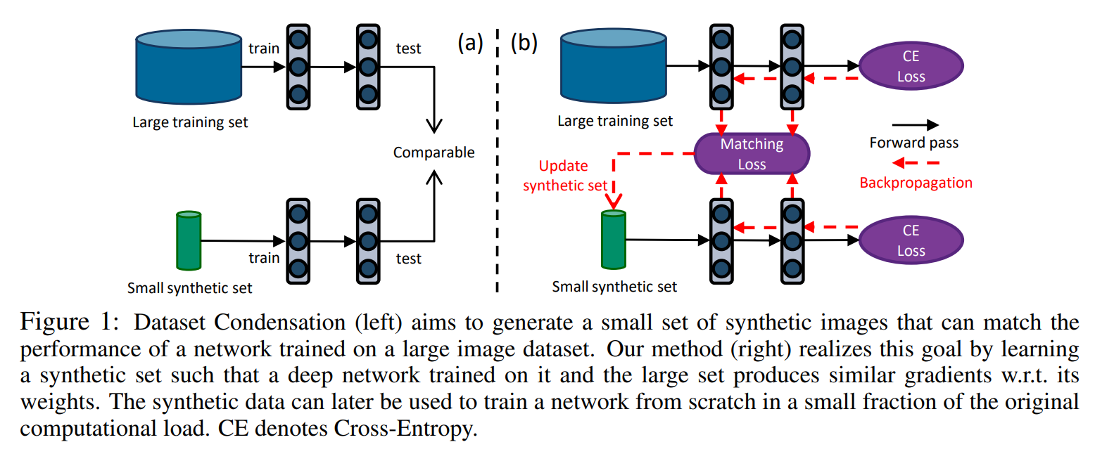
• Dataset Distillation을, 전체 학습 데이터와 소수의 합성 데이터에서 학습된 신경망 가중치의 gradient 간의 일치 문제(gradient matching problem)로 정식화함.

 

 

Introduction

• 대규모 데이터를 효과적으로 처리하는 전통적인 방법은 coreset construction이며, 이는 *클러스터링 기반의 접근법을 사용함. 또한, continual learning이나 active learning을 통해 대규모 데이터를 효율적으로 다루려는 연구도 활발히 진행되고 있음.
• 이러한 방법들은 일반적으로 대표성을 정의하는 기준(e.g., diversity, representation 등)을 먼저 설정하고, 해당 기준에 따라 대표 샘플을 선택한 뒤, 선택된 소규모 데이터셋으로 downstream 작업(e.g., classification 등)을 위한 모델을 학습함.
• 그러나 이러한 접근법들은 heuristic에 의존하기 때문에 downstream 작업에 대해 최적이라는 보장이 없으며, 실제로 대표성 있는 샘플이 존재한다는 것도 보장되지 않음.
• 본 논문은 이러한 한계를 극복하기 위해, 대규모 원본 데이터와 소규모 합성 데이터로부터 학습된 신경망의 gradient 간 차이를 최소화하는 gradient matching 기반의 dataset distillation 방법을 최초로 제안함.

*전체 데이터들을 몇 개의 중심점(대표 샘플)으로 요약함.

 

 

Method

Dataset Condensation

• Deep neural network $\phi$는 전체 데이터셋 $\mathcal{T}$에 대해서 다음의 empirical loss를 최소화하여 parameter $\theta$를 최적화함.
  $$
  \theta^{\mathcal{T}} = \arg\min_{\theta} \mathcal{L}^{\mathcal{T}}(\theta);\quad \mathcal{L}^{\mathcal{T}}(\theta) = \frac{1}{|\mathcal{T}|} \sum_{(x, y) \in \mathcal{T}} \ell(\phi_\theta(x), y)
  $$
• Dataset distillation의 목적은 condensed synthetic samples $\mathcal{S}$을 만드는 것으로, 이를 통해 학습한 모델은 다음과 같음.
  $$
  \theta^{\mathcal{S}} = \arg\min_{\theta} \mathcal{L}^{\mathcal{S}}(\theta);\quad \mathcal{L}^{\mathcal{S}}(\theta) = \frac{1}{|\mathcal{S}|} \sum_{(s, y) \in \mathcal{S}} \ell(\phi_\theta(s), y)
  $$
• 이를 통해 얻은 $\phi_{\theta^\mathcal{S}}$ 모델의 일반화 성능이 $\phi_{\theta^\mathcal{T}}$의 일반화 성능과 최대한 가까워야함.
  $$
  \mathbb{E}_{x \sim P_{\mathcal{D}}} \left[ \ell\left( \phi_{\theta^{\mathcal{T}}}(x), y \right) \right] \simeq \mathbb{E}_{x \sim P_{\mathcal{D}}} \left[ \ell\left( \phi_{\theta^{\mathcal{S}}}(x), y \right) \right]
  $$
• 초기 Dataset Distillation 논문 [related post]은 모델 파라미터 $\theta^\mathcal{S}$를 synthetic data $\mathcal{S}$의 함수로 정의함. 이를 통해 최적의 synthetic images $\mathcal{S}^*$에 학습된 모델 $\theta^\mathcal{S}$이 original dataset $\mathcal{T}$에 대해서 학습 손실이 최소가 되도록 함.
  $$
  \mathcal{S}^* = \arg\min_\mathcal{S} \mathcal{L}^{\mathcal{T}}(\theta^{\mathcal{S}}(\mathcal{S})) \quad \text{subject to} \quad \theta^{\mathcal{S}}(\mathcal{S}) = \arg\min_{\theta} \mathcal{L}^{\mathcal{S}}(\theta)
  $$
• 하지만, 이는 *nested loop optimization을 포함하고 있으므로 계산 비용이 높음.

*바깥 루프에서는 합성 데이터 $\mathcal{S}$를 업데이트하고, 안쪽 루프에서는 현재 $\mathcal{S}$에 대해 $\theta_\mathcal{S}$를 새로 학습해야 함. 이때, 합성 데이터 $\mathcal{S}$의 gradient를 구하기 위해서는 내부 루프에서 전체 신경망을 다시 학습해야 함.

 

Dataset Condensation with Parameter Matching

• Parameter matching은 합성 데이터 $\mathcal{S}$에서 학습한 모델 $\phi_\theta^\mathcal{S}$이 원본 데이터에서 학습한 모델 $\phi_\theta^\mathcal{T}$와 유사한 일반화 성능을 얻을 뿐 아니라, 파라미터 공간 상에서 유사한 해 $(\theta^\mathcal{S} \approx \theta^\mathcal{T})$로 수렴하도록 유도함.
• $\phi_\theta$가 locally smooth function일 때, 유사한 weight $(\theta^\mathcal{S} \approx \theta^\mathcal{T})$는 국소 영역에서 유사한 mapping을 의미하고, 결과적으로 유사한 일반화 성능을 의미함. 이러한 목표는 다음의 식으로 표현될 수 있음.
  $$
  \min_\mathcal{S} D(\theta^\mathcal{S}, \theta^\mathcal{T}) \quad \text{subject to} \quad \theta^\mathcal{S}(\mathcal{S}) = \arg\min_{\theta} \mathcal{L}^\mathcal{S}(\theta)
  $$
• 즉, $\theta^\mathcal{S}$를 $\mathcal{S}$ 데이터에서 훈련하여 얻은 최적의 파라미터라고 할때, $\theta^\mathcal{S}$와 $\theta^\mathcal{T}$간의 거리를 최소화하여 $\mathcal{S}$를 최적화 하는 문제임.
• 위는 하나의 고정된 초기값 $\theta_0$에서 학습된 모델에 최적화된 합성데이터를 얻지만, 실제로는 랜덤 초기값에 대해서 잘 작동하는 합성데이터를 만들어야 함.
  $$
  \min_\mathcal{S} \mathbb{E}_{\theta_0 \sim P_{\theta_0}} \left[ D(\theta^\mathcal{S}(\theta_0), \theta^\mathcal{T}(\theta_0)) \right]
  \quad \text{subject to} \quad
  \theta^\mathcal{S}(\mathcal{S}) = \arg\min_{\theta} \mathcal{L}^\mathcal{S}(\theta(\theta_0))
  $$
• 하지만, 이 또한 합성 데이터 $\mathcal{S}$에 따라 모델 $\theta_\mathcal{S}$를 다시 학습해야 하기 때문에, 매우 큰 계산 비용이 요구됨. 이를 해결하기 위해서, $\theta^\mathcal{S}$를 *incomplete optimization의 출력으로 재정의하는 back-optimization 접근을 활용할 수 있음.
  $$
  \theta^\mathcal{S}(\mathcal{S}) = \text{opt-alg}_{\theta}(\mathcal{L}^\mathcal{S}(\theta), \varsigma)
  $$
• 실제 구현에서는 서로 다른 초기값에 대해 $\theta_\mathcal{T}$를 미리 offline으로 학습해두고, 이를 target parameter vector로 사용할 수 있지만, 이는 아래의 두가지 문제가 있음.
  1. $\theta_\mathcal{S}$가 학습되는 중간 단계에서는 $\theta_\mathcal{T}$와의 거리가 매우 멀 수 있으며, 이 경로상에 다수의 local minimum가 존재해 도달하기 어려움.
  2. $\text{opt-alg}$ 최적화 과정은 계산 속도와 정확도 간의 trade-off로 인해 제한된 step $(\varsigma)$만 진행되므로 최적해에 도달하기 어려움.

*최적의 해를 다 찾기 전에 중간에서 멈추는 최적화, 즉 중간 몇 step까지만 최적화를 진행하고 멈춤.

 

Dataset Condensation with Curriculum Gradient Matching

• Parameter matching의 문제를 해결하기 위해 curriculum 기반의 방법을 제안하여, $\theta^\mathcal{S}$가 최종 $\theta^\mathcal{T}$와 가까워지는 것뿐만 아니라, *$\theta^\mathcal{S}$와 비슷한 경로를 따르도록 함.
  $$
  \min_\mathcal{S} \mathbb{E}_{\theta_0 \sim P_{\theta_0}} \left[ \sum_{t=0}^{T-1} D(\theta_t^\mathcal{S} , \theta_t^\mathcal{T}) \right]
  \quad \text{subject to} $$ $$
  \theta_{t+1}^\mathcal{S}(\mathcal{S}) = \text{opt-alg}_\theta(\mathcal{L}^S(\theta_t^\mathcal{S}), \varsigma^\mathcal{S})
  \quad \text{and} \quad
  \theta_{t+1}^\mathcal{T} = \text{opt-alg}_\theta(\mathcal{L}^\mathcal{T}(\theta_t^\mathcal{T}), \varsigma^\mathcal{T})
  $$
• 이를 통해, 매 iteration마다, 합성데이터 $\mathcal{S}$로 학습된 파라미터 $\theta^\mathcal{S}_t$가 원본데이터로 학습된 파라미터 $\theta^\mathcal{T}_t$와 유사하도록 합성데이터 $\mathcal{S}$를 학습하게 됨.
• $D(\theta^\mathcal{S}_t, \theta^\mathcal{T}_t) \approx 0$을 통해서, $\theta^\mathcal{T}_t$를 $\theta^\mathcal{S}_t$로 대체하고 $\theta^\mathcal{S}$를 $\theta$로 표기하면 다음과 같이 단순화할 수 있음.
  $$
  \theta_{t+1}^\mathcal{S} \leftarrow \theta_t^\mathcal{S} - \eta_\theta \nabla_\theta \mathcal{L}^S(\theta_t^\mathcal{S})
  \quad \text{and} \quad
  \theta_{t+1}^\mathcal{T} \leftarrow \theta_t^\mathcal{T} - \eta_\theta \nabla_\theta \mathcal{L}^T(\theta_t^\mathcal{T})
  $$ $$
  \min_S \mathbb{E}_{\theta_0 \sim P_{\theta_0}} \left[ \sum_{t=0}^{T-1} D\left( \nabla_\theta \mathcal{L}^S(\theta_t), \nabla_\theta \mathcal{L}^T(\theta_t) \right) \right].
  $$
• 즉, 모델 파라미터 $\theta$에 대한 원본데이터 loss와 합성데이터 loss의 gradient를 일치시키도록 $\mathcal{S}$를 업데이트할 수 있음. 이를 통해, *이전 파라미터들에 대한 계산 그래프를 unroll할 필요가 없다는 장점이 있음.

*$\theta$가 자유롭게 최적화되는 걸 제한할 수 있지만, 원하는 방향으로 수렴하도록 최적화 방향을 더 잘 안내해주고, step 수가 적은 optimization이라도 좋은 결과를 얻을 수 있음.

 

*기존 방법은 모델 파라미터가 여러 스텝에 걸쳐 업데이트되는 전체 과정을 추적해야 하며, 그 경로에 따라 역전파를 적용할 수 있도록 계산 그래프를 풀어서(unroll) 저장해야 함. 즉, $(\theta_1 \rightarrow \theta_2 \rightarrow \dots \rightarrow \theta_T)$. 따라서 이는 시간과 메모리 소모가 큼.

반면, gradient mathcing 방법은 현재 시점의 파라미터에 대한 gradient만 계산하면 되므로, 파라미터 경로를 역추적하거나 저장할 필요가 없음. 즉, 계산 그래프를 unroll할 필요가 없음.

Algorithm

1. 합성데이터가 다양한 초기 모델에서도 잘 작동하도록, outer loop에서는 매번 $\theta$를 무작위로 초기화한 뒤 그에 맞춰 합성데이터를 학습시킴.
2. $\theta$가 무작위로 초기화되면, 원본데이터에 대한 loss $\mathcal{L}^\mathcal{T}$와 합성데이터에 대한 loss $\mathcal{L}^\mathcal{S}$을 구하고, $\theta$에 대한 gradient를 구함
3. gradient $\nabla_\theta\mathcal{L}^\mathcal{S}$를 $\nabla_\theta\mathcal{L}^\mathcal{T}$와 가깝도록 합성데이터 $\mathcal{S}$를 최적화함.
   • 매 iteration마다, 하나의 클래스에 해당하는 샘플로만 원본데이터와 합성데이터 손실함수를 계산하며, 각 클래스에 대한 합성데이터를 병렬적으로 업데이트함.
   • 여러 클래스를 동시에 흉내내는 것 보다, 단일 클래스에 대해 평균 gradient를 모방하는 것이 더 쉬움.
4. 업데이트된 합성데이터를 사용하여, Loss $\mathcal{L}^\mathcal{S}$가 최소화되도록 $\theta$를 학습시킴.

Gradient mathcing loss

• $\phi_\theta$가 multi-layered neural network 이므로, matching loss $D$를 layerwise loss $d$의 합으로 표현할 수 있음.
  $$
  D(\nabla_\theta \mathcal{L}^\mathcal{S}, \nabla_\theta \mathcal{L}^\mathcal{T}) = \sum_{l=1}^{L} d(\nabla_{\theta^{(l)}} \mathcal{L}^\mathcal{S}, \nabla_{\theta^{(l)}} \mathcal{L}^\mathcal{T})
  $$ $$
  d(\mathbf{A}, \mathbf{B}) = \sum_{i=1}^{\text{out}} \left( 1 - \frac{\mathbf{A}_i \cdot \mathbf{B}_i}{\|\mathbf{A}_i\| \|\mathbf{B}_i\|} \right)
  $$
  • $\mathbf{A}_i, \mathbf{B}_i$는 각 출력 노드 $i$에 해당하는 gradient를 flatten한 vector임.

 

Experiments

Dataset Condensation

• 합성데이터는 Gaussian nosie로부터 초기화되거나 원본데이터에서 무작위로 선택됨.
• Dataset condensation은 합성데이터를 학습하는 단계 ($\text{C}$)와 이 합성데이터에 classifer를 학습하는 단계 $(\text{T})$의 두 단계로 이루어져 있음.
• 실험평가를 위해, 첫번 째 단계에서는 5개의 합성데이터를 생성하고, 두번 째 단계에서는 각 합성데이터에 대해서 20개의 무작위로 초기화된 모델이 학습됨. 즉, 100개의 모델이 평가됨.

Cross-architecture generalization

• 본 논문에서 제안한 방법은 하나의 네트워크 구조에서 학습된 합성이미지를 다른 네트워크 구조를 학습하는 데에도 사용할 수 있다는 장점이 있음. Table 2는 다양한 모델을 대상으로, 합성이미지가 구조에 상관없이 잘 작동한다는 것을 보여줌.

 

Applications

Continual Learning

Neural Architecture Search

• Dataset Distillation으로 합성한 이미지를 활용하면, 다양한 모델을 빠르게 학습시키고 성능을 검증하여 최적의 구조를 효율적으로 얻을 수 있음.

 

 

Conclusion

• 본 논문은 최초의 gradient matching 기반 dataset distillation 방법을 제안함.
• 제안된 방법으로 생성된 이미지들은 특정 모델 구조에 종속되지 않기 때문에, 서로 다른 구조의 모델들을 학습하는 데에도 활용될 수 있음.
• ImageNet처럼 복잡하고 고해상도의 데이터셋으로 확장할 필요가 있음.